
Detecting Changes in Product Quality After a Process Change

A common problem in manufacturing is to determine if a process change affects the quality of a product. The problem then is to compare two populations experimentally and decide whether differences that are observed are genuine or merely due to chance. This raises an important question about the choice of a relevant reference distribution. A recent experience I had with a colleague serves as a useful illustration.
A change was made to the production of a raw material used in our manufacturing process. This raw material is used to process our finished products and is not a component of the product itself. Extensive testing showed that the material properties of the raw material were not affected, so the decision was made to implement the change. As a precaution, we measured a substitute quality characteristic of three finished products per batch for 42 weeks prior to the change and 6 weeks after the change.
A colleague chose to conduct a hypothesis test on the mean values of the substitute quality characteristic before and after the change. A plot of the data is shown in Figure 1. The mean value before the process change (Process A) was 1456 [1449-1464, 95%, N=4230]. The mean value after the process change (Process B) was 1522 [1473-1527, 95%, N=90]. The difference in means was 66 with a t-statistic of 2.6. The probability of a t-statistic of 2.6 or larger is 0.0048 (p = 0.0048). Thus my colleague rejected the null hypothesis that the means were not different, and concluded that the difference between Process A and B was genuine and not due merely to chance. However, because of the considerable variability in the measurements before the change, my colleague wondered whether this analysis method was valid.
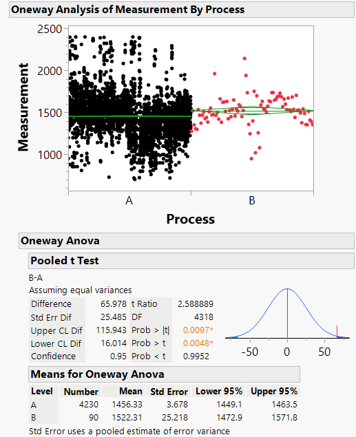
In order for the hypothesis test as conducted to be valid, the measurements from Process A (the reference set) should be normally, identically, and independently distributed relative to measurements from Process B. If these assumptions are not true, then the data from Process A is an inappropriate reference set.
An elegant method of constructing a relevant reference set is described in Statistics for Experimenters by Box, Hunter and Hunter. They propose using the 4230 measurements made before the change to determine how often in the past had differences at least as great as 66 (the difference in means between Process A and B) occurred between averages of successive groups of 90 (the number of parts measured for Process B). The distribution of these 4141 differences between averages of adjacent sets of 90 observations is shown in Figure 2. These differences provide a relevant reference set with which the observed difference of 66 (red line in Figure 2) may be compared. In this case, a difference of 66 or greater was observed 803 times.
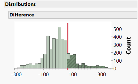
We can say that, in relation to this reference set, the observed difference was statistically significant at the 803/4141 = 0.19 level of probability (p = 0.19). In other words, the probability of observing a difference of 66 or larger merely by chance is 19%, which provides little evidence against the null hypothesis that the observed difference is part of the reference set. Thus the difference observed by my colleague was not large enough to conclude that there was a change in the product quality.
Unlike the original hypothesis test, this approach does not require the data to be independent or normal. It only assumes that whatever mechanisms gave rise to the original observations (Process A) are operating after the change (Process B). As such, it is a useful technique for comparing two populations.
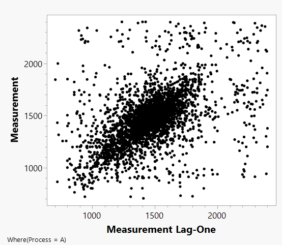
But why are the probabilities for the null hypothesis so different between these two methods (p = 0.0048 compared to p = 0.19)? Figure 3 shows a plot of each measurement versus the adjacent previous measurement. The plot shows a clear auto-correlation of adjacent observations in the Process A data. The positive autocorrelation in these data produces an increase in the standard deviation. Thus the reference distribution in Figure 2 has a larger spread than the corresponding scaled t distribution in Figure 1. The student’s t test gives the wrong answer because it assumes that the errors are independently distributed, which, as shown in Figure 3, they are not.
Because of influences such as serial correlation, the t test based on normal, independent, and identically distributed assumptions will not be valid. A very useful method for resolving this problem is to generate an external reference distribution from the past data as described above.
If you do not have access to past data, you might be able to use a randomization distribution from the results of a randomized experiment to supply a relevant reference set. This method was originally proposed by Ronald Fisher in his 1935 book The Design of Experiments and further outlined in Statistics for Experimenters.